Multi Dimensional Scaling
Multi Dimensional Scaling (MDS) is very similar to Principal Component Analysis (PCA), except that instead of converting correlations into a 2D graph, it converts distances among the samples into a 2D graph.
Definition
Imagine that you have ten runners and their measured performance for ten races. You want to visualize on a 2D graph the similarity (or dissimilarity) of the performances of the different runners. Multi Dimensional Scaling is a method to compute coordinates for each item in a chosen number of dimensions (usually 2D) so that the distances between points match the dissimilarities between items as closely as possible.
- In other word we calculate for each ${\binom{10}{2} = 45}$ pairs of runners, a distance or dissimilarity based on their results on each race. The results are stored in a dissimilarity matrix.
- These distances are then computed using a stress function that minimize the difference between interpoint distance on the graph and the actual distance calculated in the dissimilarity matrix.
- We plot the 2D coordinates: runners with similar performance end up close and those with different performance end up far. Note that MDS can also be used on greater dimension (3D, 4D, ...).
Let's calculate Euclidian distance for our dissimilarity matrix:
$$ \text{Euclidean Distance}(v, w) = \sqrt{\sum_{i=1}^{n} (v_i - w_i)^2} $$
- ${(v, w)}$ pair of two items ${v}$ and ${w}$ (e.g two runners we compare)
- ${i}$ the values to compare (e.g the measured performance ${v_i}$ and ${w_i}$ for runners ${v}$ and ${w}$ for the race ${i}$)
Then MDS minimize the calculated distances for each pair in order to plot them together on a 2D graph:
- Given distances ${d_{ij}}$ between any runners ${i}$ and ${j}$
- Find positions ${(x_{ij}, y_{ij})}$
- With 2D space ${k = 2}$
- That minimize a stress function
$$ \sum_{k=1}^{k=2}\sum_{i}\sum_{j} (|x_{ik}-x_{jk}| - d_{ij})^2 $$
⚠️ When the dissimilarities are Euclidean distances, MDS gives the same coordinates of points as PCA. This is because minimizing the Euclidean distances between points is equivalent to maximizing their linear correlations.
There are all distances you can compute with rdist in R:
Manhattan distance
$$ d(x,y) = \sum_{i=1} |x_i - y_i| $$
- Counts the total absolute differences.
- Useful when you care about additive differences e.g distance between genotypes
Canberra distance
$$ d(x,y) = \sum_{i=1} \frac{|x_i - y_i|}{|x_i| + |y_i|} $$
- Normalizes the difference by the magnitude of the values.
- Sensitive to small change near zero
- Useful for data with many zeros e.g. allele frequencies in populations.
Binary distance (Jaccard)
$$ d(x,y) = \frac{r + s}{q + r + s} $$
- Where ${q}$ number of cases where ${(x = 1 ; y = 1)}$
- Where ${r}$ number of cases where ${(x = 1 ; y = 0)}$
- Where ${s}$ number of cases where ${(x = 0 ; y = 1)}$
- Measure dissimilarity between presence/absence data
- Ignore absence/absence case
- Useful for presence/absence data e.g. grid of regions with observed species or not within
Maximum distance (Chebyshev)
$$ d(x,y) = \max_{i} |x_i - y_i| $$
- Only capture largest single difference
- Useful if the worst-case difference dominates e.g. nucleotide pair read quality control
Example of distance between genotypes
Data set
We work on a collection of 10 tetraploid genotypes and 10,000 SNPs. We want to visualize how close the genotypes are on a 2D graph.
vcf <- read_tsv(file="example.vcf")
| SNP_ID | A | B | C | D | E | F | G | H | I | J |
|---|---|---|---|---|---|---|---|---|---|---|
| SNP00 | 0 | 1 | 0 | 0 | 1 | 1 | 1 | 0 | 0 | 0 |
| SNP01 | 4 | 4 | 0 | 0 | 1 | 0 | 1 | 0 | 4 | 4 |
| SNP02 | 0 | 2 | 3 | 2 | 2 | 3 | 2 | 3 | 0 | 0 |
| ... | ... | ... | ... | ... | ... | ... | ... | ... | ... | ... |
| SNP9999 | 2 | 0 | 4 | 4 | 1 | 4 | 1 | 4 | 2 | 2 |
Dissimilarity Matrix
A dissimilarity matrix is a table that shows the distance between pairs of vectors. Here our vectors are genotypes observed on 10,000 SNPs. We use Manhattan measure to compute distances between genotypes. We observe 5 classes of genotypes 0,1,2,3,4. For a given pair ${(v, w)}$ of observed genotypes ${i}$, the maximum distance is 4 - 0 = 4 and the minimum distance is 0.
$$ \text{Manathan Distance}: \sum_{i} |v_i - w_i| $$
As we cannot process missing data, we remove SNPs with missing calls so that we keep 9,000/10,000 SNPs to generate the dissimilarity matrix.
In R, you need rdist function from the rdist R package to compute pairwise distances.
vcfDist <- rdist::rdist(t(vcf[,-1] %>% na.omit) , metric= "manhattan")
dst <- data.matrix(vcfDist)
colorsLevels =hcl.colors(100, "Inferno")
dimDst <- ncol(dst)
par(mar = c(5, 5, 5, 5))
fields::image.plot(1:dimDst, 1:dimDst, dst, axes = FALSE, xlab="", ylab="", col=colorsLevels)
axis(1, 1:dimDst, row.names(dst), cex.axis = 0.7, las=3)
axis(2, 1:dimDst, colnames(dst), cex.axis = 0.7, las=1)
This is a plot of the pairwise manhattan distance between genotypes. The lighter the greater the distance.

Multi dimensional scaling
We want to visualize genotypes distance in the dissimilarity matrices as a set of geometry points. Here the term distance is standing for measure of dissimilarity. We want to project our manhattan distances in an euclidian space of 2 dimensions. We use classic multi dimensional scaling to produce 2D-coordinates from manhattan distance values.
- Given distances ${d_{ij}}$ between genotypes ${i}$ and ${j}$
- Find positions ${(x_{ij}, y_{ij})}$
- With maximum dimension of the space which the data are to be represented in ${k = 2}$
- That minimize a stress function
$$ \sum_{k=1}^{k=2}\sum_{i}\sum_{j} (|x_{ik}-x_{jk}| - d_{ij})^2 $$
In base R, MDS is available as cmdscale function.
fit <- cmdscale(vcfDist, eig = TRUE, k = 2)

fitVcfDistDf <- data.frame(
  genotype = row.names(fit$points),
  x = fit$points[, 1],
  y = fit$points[, 2]
)

ggplot(fitVcfDistDf, aes(x = x, y = y, label = genotype)) +
  geom_point() +
  geom_text(hjust = 0, vjust = 0) +
  theme_minimal() +
  xlim(-4000, 16000) +
  xlab("") +
  ylab("")
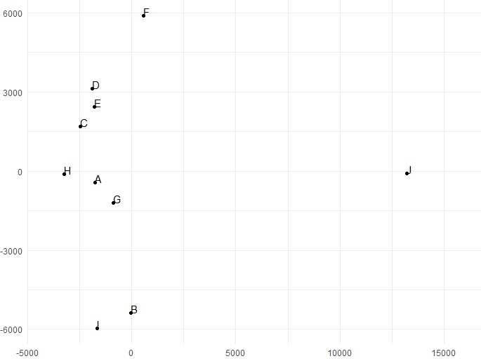
The MDS reveals that the genotypes J and F are distinct from the rest of the samples.
Conclusion
- PCA creates plots based on correlations among samples. It is a visualization of variance.
- MDS create plots based on distances or dissimilarity among samples. It is a visualization of similarity.
References
Multidimensional scaling for large genomic data sets
Jengnan Tzeng, Henry Horng-Shing Lu and Wen-Hsiung Li
BMC Bioinformatics, 2008. DOI: 10.1186/1471-2105-9-179
Multidimensional scaling: I. theory and method.
Warren S Torgerson
Psychometrika, 1952. DOI: 10.1007/BF02288916
Relevant Tags
About the Author
Latest Articles
-
Research Tax Credit
The Research Activities Tax Credit is a tax credit that incentivizes private companies to increase their Research and Development (R&D). Within my company, I have been tasked with writing the Research Tax Credit (CIR) justification report for France. Here, the method for writing such a report.OCT 2025 · PIERRE-EDOUARD GUERIN -
Turing Complete: From Logical Gates to CPU Architecture
In 2021, LevelHead published Turing Complete, a game about computer science. My friend Christophe Georgescu recommended me to play it. Unfortunately, I took his advice and now I can not stop to play this game! The game challenges you to design an entire computer from scratch. You start with basic logic gates, then move on to components, memory, CPU architecture, and finally assembly programming. By the way, the game is neat and present all these concepts in a playful and intuitive way.SEP 2025 · PIERRE-EDOUARD GUERIN -
How to Manage a Project?
In any company, every task is part of a project. I am responsible for managing multiple projects each year. I have to present deliverables to stakeholders, meet deadlines, allocate mandays and coordinate everyone’s actions. This is a meticulous work that requires a strong methodology.JUN 2025 · PIERRE-EDOUARD GUERIN